Fundamentals
Cross-cutting concepts that apply across multiple analytics functions.
Most analyses in aedifion.analytics share a small set of underlying concepts — what counts as a reference vs. an analysis period, how savings are derived, and how raw consumption is corrected for weather. Rather than restate them in every algorithm description, this page is the canonical reference. Individual algorithms in Algorithms link back here.
Analysis period and reference period
Several analyses contrast two time windows:
- The analysis period is the time window the analysis is currently evaluating — typically the most recent calendar week or month.
- The reference period is an earlier window used as a baseline. Depending on the analysis it represents either historical operation (before an optimization measure was applied) or a model-fit window used to characterize the building's behavior.
The reference period is configured per instanced component via component attributes. For buildings the relevant attributes are B+REFE_STRT / B+REFE_STOP; for air handling units AHU+REFE_STRT / AHU+REFE_STOP — see Component models. Several B+REFE_* attributes additionally let users override the reference room temperature, heating limit, and cooling limit.
Analyses that rely on a reference period include Heat Demand, Temperature Efficiency and Temperature Adjustment Savings.
Savings potential
Several analyses in the platform report a savings potential alongside their findings — energy, financial, and CO2 figures that say "if the issue this analysis just flagged were corrected, this is roughly what you would save."
Throughout this document, counterfactual refers to the estimated state of the building if a detected deviation had not occurred: same period, same conditions, but under optimal operation.
A savings potential is a counterfactual estimate, not a measurement. It is not a refund, not a guarantee, and not money that already moved. It is the platform's best answer to a single recurring question:
How much energy, money, and CO2 would have been saved during the reporting period if the deviation that this analysis detected had not occurred?
The shared pattern
Every analysis that reports savings follows the same four steps. Only the first one differs between analyses; the rest are common.
- Detect a deviation between observed operation and an expected / optimal operation. The "deviation" is the analysis-specific part: a room temperature off its optimal setpoint, a duct pressure off its setpoint, a fan running outside its declared schedule, or a heat-recovery system not extracting all the energy it could.
- Quantify the energy delta between the observed period and the counterfactual period, in kilowatt-hours, integrated over the analysis window. This is what would not have been consumed (or would have been recovered) under the optimal operation.
- Convert the energy delta into financial and CO2 figures by multiplying it by per-energy-type prices and emission factors.
- Extrapolate the analysis period KPIs to a full year. Since most analyses run on reporting windows shorter than a year (typically a week or month), the analysis period values are scaled up to annual estimates. The yearly figures are usually the headline numbers: they are directly comparable across analyses and across buildings, and they are what most users care about when prioritizing measures or estimating ROI. See From the period to a year for the extrapolation methods.
The result is always a triple: an energy number in kWh, a financial number in €, and a CO2 number in kilograms — reported both for the reporting period and as a yearly estimate. The three units describe the same physical delta; they are not independent estimates.
The three KPIs
For each savings-producing analysis you will see, per energy type (electricity, heat, cold), three KPIs whose names start with "savings potential" (English) or "Einsparpotential" (German):
| KPI | Unit |
|---|---|
savings potential.energy.<type> | kilowatt-hours |
savings potential.financial.<type> | euros |
savings potential.CO2 emissions.<type> | kilograms |
Most analyses also report a yearly version (yearly savings potential.…) that scales the analysis period KPIs up to a full year (see From the period to a year below). The platform additionally emits aggregate total yearly savings potential KPIs that combine all energy types from a given analysis.
Where prices and emission factors come from
Each analysis resolves a price and a CO2 factor per energy type (electricity, heat, cold). The lookup uses the first source that has a value:
- The analyzed component — an explicit attribute on the AHU, fan, or meter the analysis runs against.
- The building — the same attribute at building scope (the common case for site-wide tariffs and emission factors).
- A library default — a generic value declared on the abstract component definition, used so a savings KPI can always be produced even on lightly-configured projects.
Values from the first two sources are site-specific; values from the default are generic estimates. Setting the attributes on the building is the easiest way to improve accuracy across all savings KPIs.
From the period to a year
Most analyses run on a reporting window shorter than a year, so the analysis period KPIs are also extrapolated to an annual estimate. Two patterns are in use:
- Time-proportional extrapolation — the period's savings are scaled by the share of the year the period covers (or by the share of scheduled hours, when the analysis is schedule-driven). Used by most analyses.
- Climate-normal extrapolation — used by the Temperature Efficiency and Temperature Adjustment Savings. Instead of scaling by elapsed time, it uses degree-hour totals from a typical climate year, so the yearly figure reflects a typical year's seasonal weighting rather than the specific weather that happened to fall inside the reporting window. The mechanics of degree-hour normalization are described in Weather normalization.
Where each analysis's deviation comes from
The list below identifies, for every savings-producing analysis, what the observed and counterfactual sides of the comparison are. If you see a savings KPI in the platform UI, this is what the underlying delta represents.
- Temperature Adjustment Savings. Compares the building actually operating at its measured room temperatures against a counterfactual in which it operated at the optimal setpoint. The energy delta is weighted by heating and cooling degree-hours from a climate-normal year, so the yearly figure is robust against unusually mild or harsh reporting periods. Reports heating, cooling, and (optionally) electricity savings.
- Setpoint Deviation. Compares the controlled variable at its measured value against a counterfactual in which it tracked its setpoint exactly. The analysis runs on many setpoints, but a savings KPI is only emitted for the subset whose deviation has a direct energy cost — see the algorithm page for the supported setpoints and the physical mechanism in each case. The reported energy savings are the net of energy that could have been saved (when the measured value exceeded the setpoint) and energy that would have been required (when it fell short).
- Setpoint Check. Compares the component running at its currently configured setpoint against a counterfactual in which it ran at the optimal setpoint declared via attributes. Reports electric or thermal savings depending on which setpoint is being checked — see the algorithm page for the supported setpoints and the physical mechanism in each case.
- Schedule. Compares the component running on its measured operating pattern against a counterfactual in which it ran only inside its declared schedule. Off-schedule runtime translates into energy savings — electric, heating, and/or cooling, depending on what the component does outside its scheduled hours.
- Temperature Efficiency. Compares the heat recovery system performing at its measured effectiveness against a counterfactual at higher effectiveness. The unused recovery potential is converted to a thermal energy delta and valued as reduced heating demand.
Assumptions and limitations
The savings figures are useful for prioritizing action, but they rest on modelling assumptions that should be kept in mind when interpreting them.
- Potential is a model, not a measurement. Each analysis assumes the deviation it detected is fully correctable, and that consumption is linear in the modelled driver (degree-hours, the cubic pressure law, schedule on/off, heat-recovery effectiveness, …). Real buildings deviate from these idealisations.
- Yearly extrapolation assumes representativeness. The time-proportional version assumes the reporting period is a fair sample of the year; the climate-normal version assumes a typical climate. Neither survives a reporting period that was, for example, the only month the fan was switched on.
Quick reading guide
| You see… | It means… |
|---|---|
| A "savings potential" KPI | Counterfactual estimate over the reporting period — what would have been saved had the deviation not occurred. Not a billed amount. |
| A "yearly savings potential" KPI | The same idea scaled up to a full year, either time-proportionally or via climate-normal degree-hours. |
| Three KPIs together (energy / financial / CO2) | Three views of the same physical delta. The financial and CO2 figures come from multiplying the kWh delta by site or default prices and emission factors. |
Weather normalization
Some energy KPIs in the platform are reported in two flavours: the raw measured value and a weather-normalized value.
Why normalize at all?
A building's heating and cooling energy use depends strongly on the weather during the reporting period. A mild winter or a cool summer can make consumption look better than it really is, while a harsh season can make genuine efficiency improvements invisible. Weather normalization removes that confounding effect by answering:
How much energy would this building have used during the reporting period if the weather had been "typical" for the location, instead of what we actually measured?
Normalized KPIs are therefore the right number to use when:
- comparing the same building year over year,
- comparing different buildings at different sites,
- judging whether an efficiency measure (insulation, control change, setpoint tuning, …) actually reduced consumption.
The raw measured KPI remains the right number for billing, settlement, and any question about what really happened on the meter.
The method: degree-hour ratio
The platform uses the degree-hour method. The formula is:
                                        degree_hours_reference
normalized_value  =  measured_value ×  ────────────────────────
                                        degree_hours_actual
Both degree-hour totals are computed over the same reporting period as the KPI itself. Conceptually:
degree_hours_actualquantifies how much heating (or cooling) demand the actual outside temperature created during the period.degree_hours_referencequantifies how much heating (or cooling) demand a typical climate year would have created during that same calendar period.
If the period was colder than typical, the reference total is smaller than the actual total and the normalized value is lower than the measured value (the building had it harder than usual; "fair-weather equivalent" use is less). If the period was milder than typical, normalization pushes the value up.
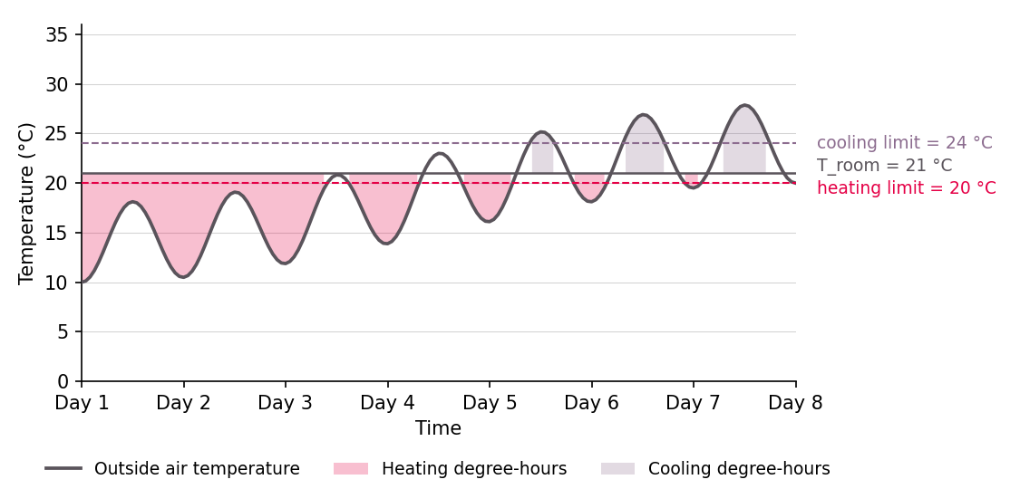
How a degree-hour is computed
For every hour in the reporting period, the platform looks at the outside air temperature and the building's reference room temperature:
- Heating degree-hours count how many degrees the outside temperature is below the room temperature, but only for hours when the outside temperature is below the building's heating limit temperature (the outdoor temperature above which the heating system is no longer expected to run). Negative differences are clipped to zero.
- Cooling degree-hours are the symmetric case: how many degrees the outside temperature exceeds the room temperature, only for hours above the building's cooling limit temperature.
These hourly contributions are then integrated over the reporting period. The unit is Degree-hours.
Building parameters
The same three building attributes are used for both the actual and the reference calculation, so the normalization isolates the weather effect. The default values can be adjusted to project specific preferences in the building component. The chosen parameters directly influence the amount of calculated degree-hours and thus the normalized consumption.
| Attribute | Default |
|---|---|
| Room air temperature | 22 °C |
| Heating limit temperature | 20 °C |
| Cooling limit temperature | 24 °C |
Where the temperatures come from
Actual outside temperature for the reporting period, in priority order
- Building's own outdoor-air temperature sensor (pin
T_AIR_ODAon the building component), if pinned. - A pinned weather station's outdoor temperature.
- A weather-service data point stored on the project.
- Weatherbit historical hourly data for the project's geographic location, as a fallback.
Reference ("typical") temperature for the same calendar period
Climate Normals long-term hourly temperature averages over 30 years for the project's geographic location.
The reference series describes one full year and is repeated/aligned to cover whatever reporting window is requested.
Which KPIs are normalized
Weather-normalized KPI-variants are produced by the relevant analyses for heating- and cooling-meters:
- Virtual Meter — aggregated value per single meter.
- Energy Consumption — total energy and per-area intensity per project.
- Energy Cost — total cost and per-area intensity per project.
- CO2 Emissions — total and per-area intensity per project.
A given meter is included in normalization only when it is configured for it. Every meter type carries the Weather normalization attribute; the choice of heating vs cooling degree-hours is implicit from the meter type, except for electricity meters where it must be set explicitly:
| Meter attribute | Applies to | Required value |
|---|---|---|
Weather normalization | All energy meters | true — switches normalization on for this meter. |
Energy application | Electricity meter (ELM) only | "heating-app" or "cooling-app" — selects which set of degree-hours (heating or cooling) drives the correction. Heat, gas, and cold meters infer this from their meter type. |
Meters tagged for other end uses (e.g. plug loads, lighting, domestic hot water) are not normalized, because their consumption is not weather-driven. Note that the normalized total may combine weather-normalized and non-normalized meter data — meters with weather-independent consumption profiles (e.g. plug loads, lighting) are included as-is.
Assumptions and limitations
The degree-hour method is a transparent, industry-standard approach, but it makes simplifying assumptions you should keep in mind when interpreting the numbers:
- Outside temperature only. Solar gains, wind, humidity, occupancy patterns, and internal loads are not corrected for. Two periods with the same degree-hour total can still differ in real demand.
- Constant building parameters. The reference room temperature and the heating/cooling limit temperatures are taken to be the same for the reference and actual calculation. If the building's setpoints or operating hours actually changed during the period, that change shows up in the normalized value (which is usually what you want — but it's not "weather only").
- Reference climate is fixed. Using climate normals (multi-year averages) rather than the specific previous year means normalized values are stable over time; they do not chase a moving baseline.
- Zero-degree-hour periods cannot be normalized. If the actual or reference period had no relevant degree-hours at all (e.g. a heating-meter KPI computed entirely over a hot summer week), normalization is skipped and only the raw value is shown.
Quick reading guide
| You see… | It means… |
|---|---|
| Normalized > measured | The reporting period was milder than typical for the site; raw consumption was flattered. |
| Normalized < measured | The reporting period was harsher than typical; the building actually performed better than the raw number suggests. |
| Normalized ≈ measured | Weather during the period was close to typical; the raw value already reflects normal conditions. |
| Only a measured value, no normalized one | The meter is not configured for normalization (Weather normalization, plus Energy application for electricity meters), required building attributes are missing, or the period had no relevant degree-hours. |