Algorithms
Detailed specification of aedifion.dynamics algorithms.
Standard .dynamics apps
Standard .dynamics apps are based directly on standard component models.
- Spot-based HVAC Air Pressure & Temperature (SHAPE) - A .dynamics algorithm shifting the electrical load of air handling units toward cheaper periods based on spot market prices.
- Slope Optimization for Thermal Heat Transfer (SLOTH) - A .dynamics algorithm ramping up heating supply temperature setpoints gradually to avoid load peaks.
- Spot Market Price Based Setpoint Interpolation (SPOT) - A .dynamics algorithm adjusting cooling temperature setpoints based on spot market prices.
The .dynamics apps can be tested without writing directly to the building by using a dryrun variation. In this case, a virtual data point with the calculated setpoints is generated and stored (similar to a VDP - virtual data point) to investigate the behavior of a .dynamics app. The dryrun variation only contains the observation part of a .dynamics app, so its required pins and attributes can differ from the productive variations.
🦎 Spot-based HVAC Air Pressure & Temperature (SHAPE)
In buildings where electricity is purchased via dynamic tariffs, the electricity costs of air handling units depend on when their fans run and when cooling is drawn from the chiller supplying their cooling coils. Without a price signal, fans and cooling coils run on fixed setpoints regardless of the electricity price, even though a lower duct pressure or a slightly warmer supply air is acceptable during expensive periods.
The SHAPE closes this gap by adjusting the supply air temperature setpoint and the supply and return air duct pressure setpoints of an air handling unit based on day-ahead spot market electricity prices. Prices are analyzed on a daily basis: every 15 minutes, the SHAPE rates the current price between the lowest and the highest price of the day between 5:00 and 18:00.
For the supply air temperature setpoint, the SHAPE uses the setpoint calculated by the HERO as its baseline. The HERO already determines the most efficient supply air temperature that keeps the building within the comfortable range, making full use of the heat recovery and avoiding counterproductive heating and cooling. Building on it means the price-based offset is applied to an already efficient setpoint instead of a fixed one. In cooling mode, the SHAPE raises this setpoint during the expensive periods of the day, increasing the offset continuously with the price up to a maximum of 1 K. The offset never raises the setpoint above the current outside air temperature, so the SHAPE writes the HERO setpoint unchanged while the outside air is not warmer than it. Outside cooling mode, the SHAPE writes the HERO setpoint unchanged as well.
For the supply and return air duct pressure setpoints, the SHAPE keeps the maximum pressure while the current price is below the median price of the day between 5:00 and 18:00. At or above the median price, SHAPE lowers the pressure setpoint once the price reaches the upper part of the price range. It then reduces the setpoint linearly toward the minimum pressure as the price reaches its maximum. The pressure setpoints always stay between the configured minimum and maximum.
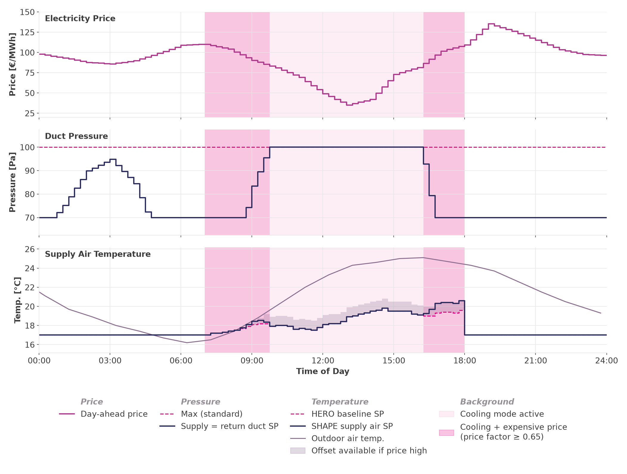
SHAPE behavior over an example day: the duct pressure setpoints stay at the maximum while the price is low and drop toward the minimum as the price rises. In cooling mode, the supply air temperature setpoint is raised above the HERO baseline during expensive periods, but never above the outside air temperature.
Choosing the duct pressure limits
The maximum pressure should be the duct pressure setpoint the building uses in standard operation, so the SHAPE never runs the fans harder than usual. The minimum pressure should be chosen as low as possible to save energy and costs, while still providing sufficient air flow to maintain comfort.
Best Practices
The SHAPE is particularly well-suited to buildings whose electricity price has a dynamic part, e.g., a dynamic tariff based on spot market prices, and to air handling units with variable-speed fans and cooling coils supplied by an electrically driven chiller, where a lower duct pressure or a slightly warmer supply air can be tolerated during expensive periods. Before implementing the SHAPE, ensure that the supply air temperature setpoint and the supply and return air duct pressure setpoints can be written and that the duct pressure setpoint attributes are configured: the maximum as the standard operating setpoint of the building, the minimum as the lowest setpoint that still maintains comfort. The SHAPE includes the HERO calculation, so the best practices of the HERO apply as well. Do not run a separate HERO on the same air handling unit, since both write the supply air temperature setpoint.
Components
Air handling unit
Default
Variation parameter: None
| Pin | Required | pin_alphanumeric_id | Input/Output |
|---|---|---|---|
| Return air temperature | Yes | EXH_T_AIR | Input |
| Outside air temperature (AHU) | Yes* | T_AIR_ODA_AHU | Input |
| Air cooler - valve - position | Yes* | C_CM+C_CRC+VAL_POS | Input |
| Supply air temperature setpoint | Yes | SUP_T_AIR_SP | Output |
| Supply air duct pressure setpoint | Yes | SUP_P_DIF_SP | Output |
| Return air duct pressure setpoint | Yes | EXH_P_DIF_SP | Output |
| Heat recovery system - position | No* | HRCS+UTIL_LEV | Input |
| Air heater - valve - position | No* | H_CM+H_CRC+VAL_POS | Input |
| Air re-heater - valve - position | No* | H_CM.RE+H_CRC+VAL_POS | Input |
| Supply air fan - operating message | No* | FAN.SUP+MSG_OPR | Input |
*: If T_AIR_ODA_AHU is not mapped, T_AIR_ODA is used instead. If a position pin is not mapped, the corresponding setpoint pin (C_CM+C_CRC+VAL_POS_SP, HRCS+UTIL_LEV_SP, H_CM+H_CRC+VAL_POS_SP, H_CM.RE+H_CRC+VAL_POS_SP) is used instead. If FAN.SUP+MSG_OPR is not mapped, FAN.EXH+MSG_OPR, MSG_OPR or COM_SWI_MN is used instead (in this order).
| Attribute | Required | Info |
|---|---|---|
| Supply air duct pressure setpoint minimum | Yes | Lowest supply air duct pressure setpoint, applied at the highest prices |
| Supply air duct pressure setpoint maximum | Yes | Highest supply air duct pressure setpoint, applied while the price is below the median price between 5:00 and 18:00 |
| Return air duct pressure setpoint minimum | Yes | Lowest return air duct pressure setpoint, applied at the highest prices |
| Return air duct pressure setpoint maximum | Yes | Highest return air duct pressure setpoint, applied while the price is below the median price between 5:00 and 18:00 |
| Supply air temperature setpoint upper limit | No | Maximum allowed supply air temperature setpoint |
| Supply air temperature setpoint lower limit | No | Minimum allowed supply air temperature setpoint |
| Return air temperature setpoint deviation tolerance | No | Allowed return air temperature above and below the ideal indoor air temperature (ideal indoor air temperature is 22°C in Winter) |
| Return air temperature setpoint maximum | No | Upper limit of the return air temperature setpoint (independent of the ideal indoor air temperature) |
| Return air temperature setpoint minimum | No | Lower limit of the return air temperature setpoint (independent of the ideal indoor air temperature) |
| Supply air fan - temperature increase | No | Supply air temperature increase due to the waste heat of the fan |
| Heat recovery system efficiency | No | Maximum efficiency of the heat recovery system |
| Heat recovery system active during cooling | No | True, if the internal control of the ahu uses the heat recovery for cooling |
| Adapt HERO parameters | No | True, if the hero is allowed to learn parameters based on the ahu behavior |
🦥 Slope Optimization for Thermal Heat Transfer (SLOTH)
In buildings supplied by heat pumps or district heating, the supply temperature setpoint is adjusted to meet the required heating power demand. In the morning, when occupancy begins, the setpoint is typically raised in a single step from night setback to the full daytime value. This step change causes a thermal power peak as the entire building must be reheated. For heat pumps, this results in expensive electrical load peaks; for district heating connections, the contracted thermal capacity can be exceeded — both leading to avoidable costs.
SLOTH closes this gap by ramping up the supply temperature setpoint gradually along a defined slope instead of raising it in a single step. This spreads the thermal power demand over time, reducing peak loads (peak shaving).
SLOTH determines a target supply temperature using a heating curve whenever the outdoor temperature used by the heating curve changes (the outdoor temperature is refreshed every 15 minutes). The heating curve relates outdoor temperature to the required supply temperature, configured via base points. To avoid overheating when outdoor temperatures rise during the day, the heating curve uses the maximum of the current outdoor temperature and the forecasted mean temperature between 8:00 and 18:00. This anticipates daytime warming and reduces unnecessary morning heating. During unoccupied periods, the target supply temperature is automatically reduced by a configurable nighttime setback.
Rather than raising the supply temperature setpoint straight to the target supply temperature defined by the heating curve, SLOTH approaches it step by step: the applied setpoint is constrained to rise by no more than 5 K per 15-minute interval above the currently measured supply temperature. This turns what would otherwise be an abrupt jump into a ramp. Once the measured supply temperature has caught up with the target supply temperature, the setpoint simply follows the target directly. The maximum increase of 5 K is a default value and can be adjusted via the "Supply temperature setpoint maximum increase per 15 min" attribute for each heating circuit.
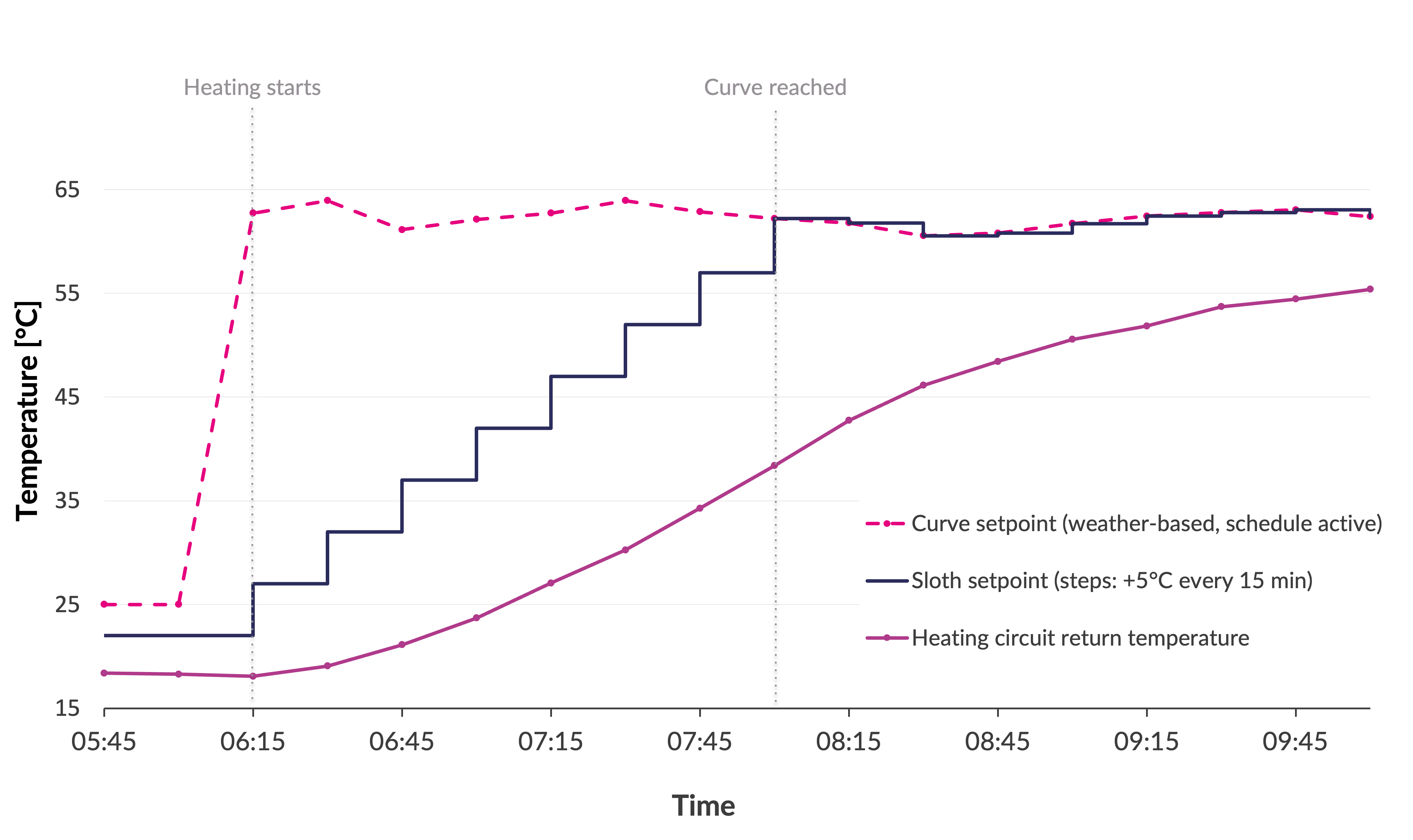
SLOTH ramp behavior: instead of raising the supply temperature setpoint to the heating curve target in a single step, SLOTH caps each 15-minute increment 5 K (default value, configurable) above the measured supply temperature, creating a gradual slope that distributes the heating power demand over time and reduces the peak load.
Caution
If an error occurs or the connection to the building is lost for longer than the alive timeout, the edge device writes the configured reset value to the supply temperature setpoint. There is no preset reset value — it must be configured explicitly, and a reset value of 30°C is highly recommended: with a high reset value, an unstable internet connection can cause the supply temperature setpoint to jump to that value in a single step, producing exactly the load peaks after the nighttime setback that SLOTH is designed to avoid.
Best Practices
SLOTH is particularly well-suited to heating circuits supplied by heat pumps or district heating connections, where load peaks at the start of the occupancy period translate directly into costs. Before implementing SLOTH:
- The supply temperature setpoint is writable
- The heating curve reference points are tuned to the building's actual heating behavior
- The occupancy schedule allows sufficient lead time for the gradual ramp-up, so comfort is achieved when occupants arrive
- A reset value is configured for the supply temperature setpoint — 30°C is highly recommended (see the caution above)
Components
Heating Circuit
Default
Variation parameter: None
| Pins | Required | pin_alphanumeric_id | Input/Output |
|---|---|---|---|
| Supply temperature | Yes | T_IN | Input |
| Supply temperature setpoint | Yes | T_IN_SP | Output |
| Attributes | Required | Info |
|---|---|---|
| Schedule | Yes | Regular schedule that is repeated every week, used to determine the occupancy period and apply the nighttime reduction outside of it. |
| Base points | Yes | The heating curve base points for the calculation. Must be given as pairs of outside air temperature/supply temperature, e.g. -12,90;20,50 |
| Night time reduction | Yes | Value (in K) subtracted from the heating curve target outside the occupancy period |
| Schedule Timezone | No | Defaults to Europe/Berlin |
| Supply temperature setpoint maximum increase per 15 min | No | Defaults to 5 K supply temperature increase per 15-minute interval |
🐆 Spot Market Price Based Setpoint Interpolation (SPOT)
In buildings where electricity is purchased via dynamic tariffs, power purchase agreements with dynamics share, or sourced from on-site PV generation, the final electricity bill and the CO2 intensity of the electricity used depend on when electricity is consumed. SPOT applies wherever such time-varying electricity prices or CO2 signals are available and the building has cooling capacity that can be shifted in time.
Electricity prices follow a daily pattern, typically peaking during morning and evening hours and having low prices in between and at night. The price spread between the cheapest and most expensive periods throughout the day can be substantial. Buildings with flexible cooling systems supplied via electricity-driven compression chillers can exploit this by pre-cooling during low-price periods and reducing cooling activity when prices are high. Without price signal integration, cooling operates on a fixed schedule and this cost-saving and CO2 emission reduction potential remains unrealized.
The SPOT algorithm closes this gap by adjusting cooling temperature setpoints based on spot market electricity prices. Prices are analyzed on a daily basis and cooling loads are shifted toward lower-cost periods, enabling systematic electricity cost reduction without compromising comfort or building operation. To achieve this, the SPOT adjusts the cooling setpoints between the minimum and the maximum supply temperature setpoints of the controlled components and selects the setpoint in order to increase cooling in cheap periods. To avoid sustained under- or over-cooling, the algorithm uses the daily median price as a midpoint reference: when the current price is below the median, the setpoint is biased toward the lower (colder) half of the range; when the price is above the median, the setpoint is biased toward the upper half. Further, in order to protect systems where the dew point of the surrounding air is relevant, the minimum setpoint can be limited by the current dew point plus a safety margin.
Best Practices
The SPOT is particularly well-suited to buildings with thermally flexible cooling systems, where pre-cooling and reduced cooling activity can be tolerated without compromising comfort. Before implementing the SPOT, ensure that the supply temperature setpoint of the cooling circuit can be written and that the minimum and maximum supply temperature setpoint attributes are configured to reflect the operational limits of the system.
Components
Cooling Circuit
Default
Variation parameter: None
| Pins | Required | pin_alphanumeric_id | Input/Output |
|---|---|---|---|
| Supply temperature setpoint | Yes | T_IN_SP | Output |
| Attributes | Required | Info |
|---|---|---|
| Supply temperature setpoint minimum | No* | Setpoint for the minimum supply temperature |
| Supply temperature setpoint maximum | No* | Setpoint for the maximum supply temperature |
| Dew point protection enabled | No | Enables dew point protection to prevent surface condensation. Values: 0 = disabled (default), 1 = enabled |
| Dew point safety margin | No | Safety margin (in K) added to the dew point when protection is enabled. Default: 1.5 K |
*: These are the attributes C_T_OUT_SP_MIN and C_T_OUT_SP_MAX of the cooling circuit, not the pins T_IN_SP_MIN and T_IN_SP_MAX of the same name.